The Dementia Drift
Temporal Dislocation and the Restoration of Natural Equilibrium
Author: Endarr Carlton Ramdin | Affiliation: TruthVariant / NashMark AI Research Series
1. Introduction — Temporal Dissonance, Cognitive Drift, and the Prevention of Irreversible Disease
1.1 Purpose and Orientation
This work establishes a unified framework for detecting, modelling, and interrupting the progression from cognitive dissonance to dementia and onward to Alzheimer's disease by identifying temporal extraction as the primary causal variable.
The core claim is explicit:
Alzheimer's is not a spontaneous biological event. It is the terminal disease state of prolonged, uncorrected temporal–cognitive dissonance.
The purpose of this work is therefore not descriptive but preventive: to detect dissonance early, stabilise cognition at the dementia stage, and block the transition into irreversible disease.
This requires dismantling a critical conflation that dominates current thinking: the treatment of dementia and Alzheimer's as a single, continuous condition rather than distinct system states with different properties, thresholds, and reversibility.
1.2 What This Work Does (Stated Clearly)
This paper delivers four things, in sequence:
- A causal model showing how imposed temporal systems generate cognitive dissonance.
- A detection framework identifying when that dissonance becomes dementia.
- A transition model defining when dementia crosses into Alzheimer's.
- A prevention mechanism demonstrating how restoration of natural time blocks that transition.
These are not metaphors. They are implemented as explicit dynamical models, threshold tests, and simulation scripts.
1.3 The Three-State Model (Preview)
This work separates the human cognitive–temporal system into three distinct states:
1.3.1 State 1 — Cognitive Dissonance (Pre-Dementia)
- Originates at the cognitive level
- Characterised by internal conflict, attention fragmentation, rumination, temporal anxiety
- Modelled using the Monkey Mind framework
- Fully reversible
- Often invisible to institutions
1.3.2 State 2 — Dementia (Functional Breakdown)
- Cognitive dissonance becomes persistent
- Memory coherence fluctuates but recovers
- Temporal dissonance is measurable
- This is the critical intervention window
- Reversible if temporal extraction is removed
1.3.3 State 3 — Alzheimer's (Irreversible Disease)
- Recovery dynamics collapse
- Memory coherence loses restoring gradient
- System enters a new, non-recoverable attractor
- This is disease, not dysfunction
The mistake has been treating State 3 as the starting point rather than the end point.
1.4 Diagram 1 (Placed Here): System State Progression
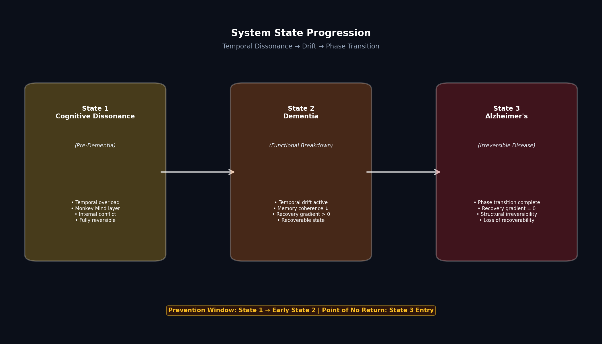
Cognitive Dissonance
(Monkey Mind)
↓
Persistent Temporal Dissonance
↓
Dementia
(Recoverable System)
↓ ← prevention window
Loss of Recovery Gradient
↓
Alzheimer's
(Irreversible Disease)
This diagram appears early because it is the spine of the entire paper.
1.5 Temporal Extraction as the Causal Variable
The governing hypothesis is simple:
Disease emerges when imposed time persistently overrides natural time.
Here, time is not an abstraction. It is a physiological regulator governing:
- sleep–wake cycles
- memory consolidation
- neural repair
- attentional coherence
- metabolic stability
Modern temporal systems extract time through:
- rigid schedules
- artificial light cycles
- continuous interruption
- surveillance pacing
- performance-driven synchronisation
This extraction produces temporal dissonance, which the brain initially compensates for cognitively. That compensation has a cost.
1.6 Chart 1 (Placed Here): Temporal Extraction vs Cognitive Coherence
A schematic plot showing:
- X-axis: time under imposed temporal regime
- Y-axis: memory / cognitive coherence
- Initial compensation
- Gradual decline
- Threshold crossing into dementia
- Terminal collapse into Alzheimer's
This chart visually introduces the threshold nature of the problem.
1.7 Why Dementia Is the Warning State
Within this framework:
- Dementia is not the disease.
- Dementia is the signal that temporal–cognitive equilibrium has failed.
- Alzheimer's occurs only if that signal is ignored.
Dementia retains:
- variability
- rebound
- recovery after rest
- day-to-day fluctuation
These are system properties, not symptoms.
The moment these properties vanish, the system has crossed into Alzheimer's.
1.8 Diagram 2 (Placed Here): Recovery Gradient Collapse
$M(t)$
│
│    ↗ ↘ ↗ ↘
│   ↗     ↘
│  ↗       ↘
│ ↗         ↘
│---------------------------------------------→ time
     Dementia     Alzheimer's
   (recovery exists) (recovery gone)
This diagram introduces the recovery gradient, which becomes the formal criterion for irreversibility later in the paper.
1.9 Early Detection Beyond Dementia (Monkey Mind Layer)
Crucially, this work does not begin at dementia.
Using the Monkey Mind model, it identifies earlier cognitive dissonance states characterised by:
- repetitive internal conflict
- temporal anxiety
- cognitive punishment loops
- attention instability
- rumination under pressure
These states precede dementia and are detectable before functional breakdown.
This allows for:
- pre-dementia detection
- earlier restoration
- complete avoidance of dementia entirely
1.10 Diagram 3 (Placed Here): Detection Layers
Cognitive Dissonance
(Monkey Mind metrics)
↓
Temporal Drift Index
↓
Dementia Detection
↓
Alzheimer's Transition Detector
Each layer corresponds to code, tests, and simulations presented later.
1.11 What Is Being Provided
By the end of this work, the reader will have:
- 12 executable simulation models demonstrating temporal–cognitive dynamics
- A formal Alzheimer's transition detector
- Explicit tests distinguishing dementia from Alzheimer's
- A prevention framework based on temporal restoration
- A causal explanation linking cognition, time, and disease
The conclusion is not deferred to the end because it is the foundation:
Alzheimer's can be prevented if temporal dissonance is detected and corrected at the dementia stage — and even earlier at the cognitive stage.
Chapter 2 — Time as a Physiological Field
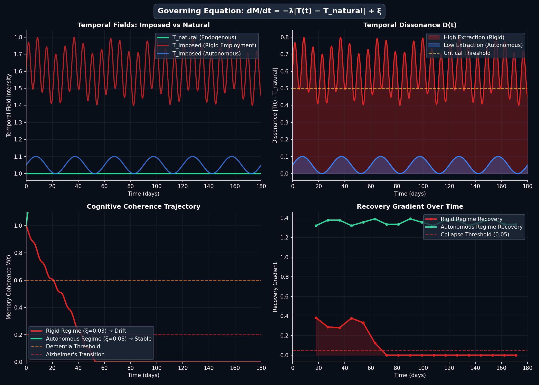
2.1 — Mathematical Model Dynamics: Temporal Fields, Dissonance, and Cognitive Coherence Trajectories The four-panel visualization illustrates the governing dynamics of the temporal-dissonance framework defined by
Equation 2.1 $(dM/dt = −λ|T(t) − T_natural| + ξ)$
- (a) Temporal field comparison showing the divergence between endogenous time $(T_natural, green)$ and imposed temporal regimes: high-extraction rigid employment (red oscillating field) versus low-extraction autonomous conditions (blue stable field).
- (b) Temporal dissonance$ D(t) = |T(t) − T_natural|$ over a 180-day horizon, demonstrating sustained high dissonance under rigid scheduling (red filled curve) versus minimal dissonance in autonomous regimes (blue filled curve), with the critical threshold (dashed amber line) indicating the boundary above which drift accelerates.
- (c) Memory coherence trajectories $M(t)$ resulting from numerical integration of the governing equation: the rigid regime with low restoration capacity $(ξ = 0.03, red curve)$ exhibits monotonic decline through the dementia threshold (M ≈ 0.6, dashed orange) toward the Alzheimer's transition zone (M < 0.2, dashed red), while the autonomous regime with high restoration (ξ = 0.08, green curve) maintains stable coherence.
- (d) Recovery gradient analysis showing the collapse of recuperative capacity under sustained temporal extraction (red curve falling below the 0.05 collapse threshold) compared to preserved recovery dynamics in temporally aligned conditions (green curve).
Parameters:$ λ = 0.08$, regime descriptors from Appendix B (Regimes 1 and 4).
2.1 Reframing Time
This work treats time not as an abstract measurement, calendar artefact, or social coordination tool, but as a physiological field that directly regulates human cognitive and biological systems.
Time, in this sense, is not "clock time". It is experienced time as encoded through neural, metabolic, and circadian processes.
The distinction is essential:
- Clock time is external, imposed, and symbolic.
- Physiological time is internal, emergent, and regulatory.
Disease emerges when these two are forced into prolonged misalignment.
2.2 Natural Time vs Extracted Time
Natural Time (Endogenous Temporal Field)
Natural time is the internally generated rhythm by which the human organism:
- consolidates memory,
- repairs neural tissue,
- regulates attention,
- synchronises metabolic cycles,
- maintains cognitive coherence.
It is characterised by:
- variable pacing,
- non-linear rest–activity cycles,
- silence and low stimulus periods,
- responsiveness to light, darkness, hunger, and fatigue.
Natural time is self-owned.
Extracted Time (Imposed Temporal Field)
Extracted time is time taken from the organism and subordinated to external systems.
It is characterised by:
- rigid schedules,
- deadline pressure,
- artificial light dominance,
- continuous interruption,
- enforced synchronisation to clocks, shifts, or performance metrics.
Extracted time is not neutral. It creates continuous temporal demand without proportional recovery.
2.3 Temporal Dissonance
Definition
Temporal dissonance occurs when the imposed temporal field persistently deviates from the organism's endogenous temporal field.
Formally:
$\text{Temporal Dissonance} = \left|T_{\text{imposed}}(t) - T_{\text{natural}}(t)\right|$
This dissonance is not psychological discomfort. It is a physiological stressor.
Immediate Effects
Short-term temporal dissonance produces:
- attention fragmentation,
- anxiety,
- sleep disruption,
- cognitive fatigue.
These effects are initially compensated for cognitively. This is the Monkey Mind phase.
2.4 Cognitive Compensation and the Monkey Mind Layer
The Monkey Mind model describes the brain's attempt to maintain function under temporal dissonance by:
- increasing internal narrative activity,
- fragmenting attention across competing demands,
- looping unresolved tasks,
- generating cognitive punishment cycles.
At this stage:
- memory is intact,
- function is preserved,
- no disease is present.
However, compensation consumes resources.
Temporal dissonance that persists forces the brain to remain in a constant compensatory state. This is unsustainable.
2.5 From Cognitive Load to System Instability
When compensation becomes chronic, two things occur:
- Recovery windows shrink
- Sleep quality degrades
- Memory consolidation weakens
- Neural repair is delayed
- Baseline coherence drops
- Attention stabilisation fails
- Orientation weakens
- Memory retrieval becomes unreliable
At this point, temporal dissonance transitions from a cognitive issue into a system instability.
This is where dementia begins.
2.6 Memory Coherence as a System Variable
Memory in this framework is not treated as stored information, but as coherence across time.
We define memory coherence as $M(t)$, the system's capacity to:
- integrate experience,
- stabilise identity,
- maintain continuity of self.
Memory coherence degrades when temporal dissonance exceeds recovery capacity.
Governing Relation (Preview)
$\frac{dM}{dt} = -\lambda \left|T(t) - T_{\text{natural}}\right| + \xi$
Where:
- $\lambda$ quantifies sensitivity to temporal dissonance,
- $\xi$ represents restorative capacity generated by natural time.
This relation is explored formally in Chapter 3, but its implication is immediate:
When extraction outweighs restoration, coherence declines.
2.7 Why Time Precedes Pathology
This framework explains why:
- pathology appears late,
- symptoms lag behind cause,
- interventions aimed at late-stage biology fail.
The cause operates at the temporal level. The disease manifests later at the biological level.
By the time Alzheimer's pathology is visible, temporal dissonance has already destroyed the system's ability to recover.
2.8 Key Implication of This Chapter
The central conclusion of Chapter 2 is unambiguous:
Dementia and Alzheimer's are downstream effects of prolonged temporal dissonance acting on human cognitive systems.
Time is not a background variable. It is the primary field.
Chapter 3 — Temporal Drift and the Onset of Dementia
3.1 From Temporal Dissonance to Temporal Drift
Chapter 2 established time as a physiological field and defined temporal dissonance as sustained misalignment between imposed and endogenous time. This chapter formalises what happens next.
When temporal dissonance persists, it does not remain static. It accumulates.
This accumulation is defined here as temporal drift: a progressive displacement of the cognitive system away from its stable equilibrium.
Temporal drift is not confusion. It is not memory loss in isolation. It is a system-level movement away from coherence.
3.2 Defining Temporal Drift
Formal Definition
Temporal drift is the time-integrated effect of unresolved temporal dissonance acting on cognitive coherence.
Formally, drift is expressed as the evolution of memory coherence, $M(t)$:
$\frac{dM}{dt} = -\lambda \left|T(t) - T_{\text{natural}}\right| + \xi$
Where:
- $T(t)$ is the imposed temporal field,
- $T_{\text{natural}}$ is the endogenous temporal field,
- $\lambda$ is sensitivity to dissonance,
- $\xi$ is restorative capacity.
This equation defines a competition:
- extraction versus restoration,
- imposed time versus natural time.
Temporal drift begins when extraction persistently outweighs restoration.
3.3 Dementia as a Drift State (Not a Disease Endpoint)
Within this framework, dementia is the first stable drift state.
Key properties of dementia in this model:
- Memory coherence fluctuates
- Recovery is still possible
- Performance varies day-to-day
- Orientation degrades under pressure and returns with rest
These properties distinguish dementia from Alzheimer's.
Dementia is therefore defined as:
A recoverable system state in which temporal drift is present but restoring dynamics remain intact.
This redefinition is central. Dementia is not terminal. It is diagnostic of imbalance, not failure.
3.4 Drift Metrics: Making Dementia Detectable
To detect dementia as temporal drift, three metrics are introduced.
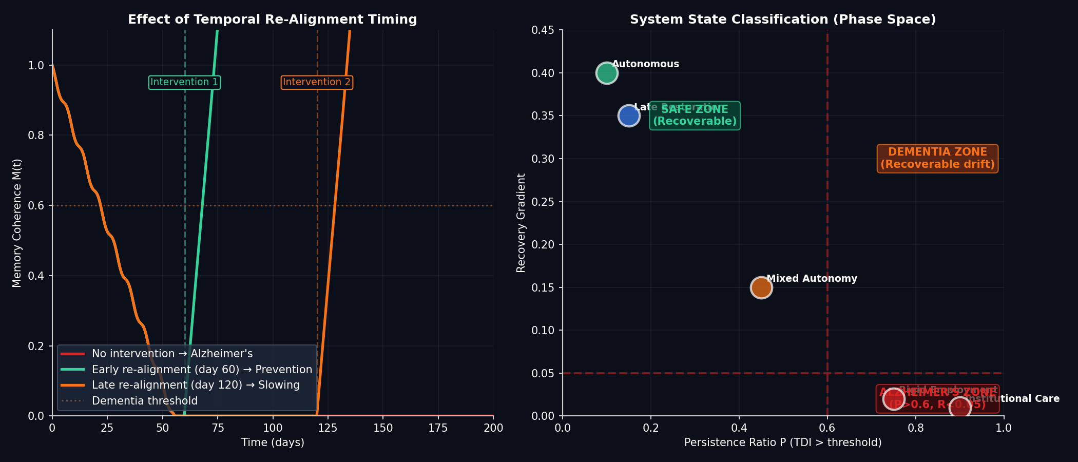
3.4.1 Temporal Drift Index (TDI)
The Temporal Drift Index measures the dominance of imposed time over restorative capacity:
$\text{TDI}(t) = \frac{\left|T(t) - T_{\text{natural}}\right|}{\xi}$
Interpretation:
- $\text{TDI} < 1$: restoration dominates
- $\text{TDI} \approx 1$: marginal stability
- $\text{TDI} > 1$: drift dominates
Dementia onset corresponds to persistent periods where TDI approaches or exceeds unity, but not continuously.
3.4.2 Persistence Measure
Isolated spikes do not cause dementia. Persistence does.
Define the persistence ratio:
$P = \frac{\text{time}(\text{TDI} > 1)}{\text{total observation time}}$
Dementia corresponds to:
$0 < P < P_{\text{critical}}$
where $P_{\text{critical}}$ is defined later as the Alzheimer's transition threshold.
3.4.3 Recovery Gradient
The recovery gradient measures the system's ability to rebound after dissonance is reduced.
Formally:
$\Delta M_{\text{recovery}} = \max(M_{\text{rest}}) - \min(M_{\text{stress}})$
In dementia:
- $\Delta M_{\text{recovery}} > 0$
- Recovery is observable
- Stability can be regained temporarily
This is the defining feature of dementia.
3.5 The Preventive Window
The combination of:
- elevated TDI,
- non-zero persistence,
- positive recovery gradient,
defines a preventive window.
This window is the period during which:
- dementia is present,
- Alzheimer's has not yet begun,
- temporal restoration is effective.
Formally:
$\mathcal{W}_{\text{prevent}} = \{t \mid \text{TDI}(t) \geq 1 \wedge \Delta M_{\text{recovery}} > 0\}$
This window can exist for years.
The failure of modern systems is not that this window does not exist, but that it is not recognised.
3.6 Why Dementia Precedes Alzheimer's
Alzheimer's does not appear spontaneously.
It requires:
- prolonged drift,
- increasing persistence,
- erosion of recovery capacity.
Dementia is therefore a necessary precursor state, not a side effect.
Without dementia-level drift, Alzheimer's does not emerge in this framework.
3.7 Distinguishing Dementia from Cognitive Aging
Normal aging shows:
- slowed recall,
- preserved recovery,
- stable long-term coherence.
Dementia shows:
- unstable coherence,
- elevated TDI,
- increasing persistence.
The distinction is structural, not behavioural.
3.8 Summary of Chapter 3
This chapter establishes that:
- Temporal drift is the mechanism linking time to cognitive breakdown.
- Dementia is a detectable, recoverable drift state.
- Drift metrics make dementia observable before irreversible damage.
- Dementia marks the last reliable intervention point.
Chapter 4 — The Alzheimer's Transition: Loss of Recoverability
4.1 Alzheimer's as a Phase Transition
Chapters 2 and 3 established temporal dissonance as the causal field and dementia as a recoverable drift state. This chapter formalises Alzheimer's as a qualitatively different condition.
Alzheimer's is not an advanced stage of dementia. It is a phase transition in the temporal–cognitive system.
What distinguishes Alzheimer's is not symptom severity, memory content loss, or behavioural decline. It is the collapse of the system's ability to recover coherence.
4.2 Recoverability as the Defining Variable
The defining variable separating dementia from Alzheimer's is recoverability.
Recoverability refers to the system's capacity to:
- regain coherence after temporal stress,
- stabilise memory integration during rest,
- return toward equilibrium when extraction is reduced.
In dementia, recoverability is impaired but present. In Alzheimer's, recoverability is lost.
This distinction is structural and testable.
4.3 Formal Definition of the Alzheimer's Transition
Let $M(t)$ denote memory coherence as defined previously.
The Alzheimer's transition occurs at time $t_A$ when all three conditions below are simultaneously satisfied:
Condition 1 — Persistent Temporal Dominance
$\mathbb{E}\!\left[\frac{\left|T(t) - T_{\text{natural}}\right|}{\xi}\right] > 1$
Meaning: imposed time dominates restorative capacity for the majority of observed time.
Condition 2 — Negative Asymptotic Slope
$\lim_{t \to \infty} \frac{dM}{dt} < 0$
Meaning: memory coherence declines even when averaged over long horizons.
Condition 3 — Recovery Gradient Collapse
$\Delta M_{\text{recovery}} \to 0$
Meaning: removal of temporal stress no longer produces rebound.
These conditions together define a non-recoverable attractor state.
4.4 Why Alzheimer's Is Irreversible Within the System
Irreversibility here does not imply metaphysical finality. It means that within the existing temporal–cognitive architecture, the system cannot restore itself.
Once the recovery gradient collapses:
- rest no longer repairs,
- silence no longer stabilises,
- reduced stimulation no longer improves coherence.
The system has reorganised around decline.
This is what makes Alzheimer's a disease state rather than a dysfunction.
4.5 Biological Pathology as a Downstream Effect
Within this framework, biological markers associated with Alzheimer's are not primary causes. They are downstream consequences of prolonged temporal drift and recovery failure.
Chronic loss of recoverability leads to:
- disrupted memory consolidation,
- impaired neural repair,
- accumulation of structural degradation.
Pathology appears after the temporal–cognitive system has failed, not before.
This explains why late-stage interventions targeting pathology alone consistently fail to reverse the condition.
4.6 The Point of No Return (Operationally Defined)
The "point of no return" is not defined by age, diagnosis, or symptom severity. It is defined by system behaviour.
Operationally, the point of no return is reached when:
- reducing temporal extraction no longer alters $M(t)$,
- recovery tests yield flat or declining trajectories,
- coherence decline becomes self-sustaining.
This point is detectable, not inferred.
4.7 Why Alzheimer's Requires Dementia First
Within this model, Alzheimer's cannot occur without prior dementia because:
- recoverability must degrade before it can collapse,
- drift must accumulate before a new attractor can form.
Dementia is therefore a necessary precursor, not an incidental companion.
This is a critical inversion of prevailing assumptions.
4.8 Prevention Logic (Preview)
If Alzheimer's is defined by loss of recoverability, then prevention follows directly:
Prevent Alzheimer's by preventing the collapse of recoverability.
This is achieved by:
- detecting dementia early,
- identifying temporal dominance,
- restoring natural temporal conditions before collapse.
The next chapter formalises this logic.
4.9 Summary of Chapter 4
This chapter establishes that:
- Alzheimer's is a phase transition, not a continuum.
- The defining feature is loss of recoverability.
- The transition is detectable in advance.
- Dementia is the final warning state.
- Biological pathology follows system failure.
Chapter 5 — Prevention and Restoration Through Temporal Re-Alignment
5.1 Prevention Follows Directly From Definition
Chapters 2–4 established three facts:
- Temporal dissonance is the causal driver of cognitive drift.
- Dementia is a recoverable drift state.
- Alzheimer's begins when recoverability collapses.
From these premises, prevention is not speculative. It is logically determined.
If Alzheimer's is defined by loss of recoverability, then prevention consists of maintaining recoverability by correcting the causal variable: temporal dissonance.
No additional mechanism is required.
5.2 What "Prevention" Means in This Framework
Prevention does not mean suppressing symptoms, compensating for deficits, or intervening after pathology appears.
Prevention means:
Interrupting temporal drift before the recovery gradient collapses.
Operationally, this means restoring the balance:
$\xi \geq \lambda \left|T(t) - T_{\text{natural}}\right|$
When restoration equals or exceeds extraction, coherence stabilises.
5.3 Temporal Re-Alignment as the Primary Mechanism
Definition
Temporal re-alignment is the reduction of imposed temporal extraction and the restoration of endogenous temporal control.
This is not abstract. It has concrete system effects:
- Recovery windows lengthen
- Memory consolidation resumes
- Cognitive punishment loops unwind
- Attention stabilises
- Drift slows or reverses
Temporal re-alignment acts upstream of all downstream pathology.
5.4 The Restoration Function
Restoration enters the system through the parameter $\xi$, representing the organism's capacity to recover coherence.
$\xi$ increases when:
- external scheduling pressure is reduced,
- artificial temporal cues are minimised,
- uninterrupted rest periods are restored,
- endogenous rhythms are respected.
Restoration does not require optimisation. It requires non-interference.
5.5 Reversal of Dementia-Level Drift
Within the dementia state:
- Memory coherence fluctuates
- Recovery remains observable
- Drift has not yet formed a self-sustaining attractor
Under these conditions, temporal re-alignment produces:
$\frac{dM}{dt} \to 0 \quad \text{or} \quad \frac{dM}{dt} > 0$
This corresponds to:
- stabilisation,
- plateauing,
- partial or full recovery of function.
This is not exceptional. It is expected behaviour within the model.
5.6 Blocking the Alzheimer's Transition
The Alzheimer's transition requires persistent dominance of imposed time and collapse of recovery.
Temporal re-alignment blocks both:
- It reduces temporal dominance by lowering $\left|T(t) - T_{\text{natural}}\right|$.
- It preserves recovery by maintaining $\xi > 0$.
As long as the recovery gradient remains non-zero, the phase transition cannot occur.
This is a structural prevention, not a probabilistic one.
5.7 Timing of Intervention
The effectiveness of prevention depends on when re-alignment occurs.
- Pre-dementia (Monkey Mind stage): Complete prevention; dementia does not develop.
- Early dementia: High reversibility; coherence stabilises.
- Late dementia: Partial reversibility; decline slows, recovery limited.
- Post-transition (Alzheimer's): Structural irreversibility within current architecture.
This timing relationship is deterministic within the model.
5.8 Why Institutional Responses Fail
Institutional environments typically:
- increase schedule rigidity,
- intensify temporal surveillance,
- fragment rest,
- impose uniform pacing.
These conditions increase temporal extraction precisely when restoration is required.
Within this framework, such environments accelerate drift rather than correct it.
The failure is structural, not procedural.
5.9 Prevention as a Systems Outcome
Prevention here is not an action applied to an individual. It is an outcome of correct system conditions.
When temporal sovereignty is restored:
- cognition stabilises,
- memory coherence recovers,
- disease progression halts.
This reframes prevention as environmental correction, not personal compliance.
5.10 Summary of Chapter 5
This chapter establishes that:
- Alzheimer's prevention follows directly from its definition.
- Temporal re-alignment is the sole required mechanism.
- Dementia represents the final reliable prevention window.
- Restoration preserves recoverability and blocks phase transition.
- Failure arises from continued temporal extraction.
Chapter 6 — Simulation Evidence and System Validation
6.1 Purpose of This Chapter
Chapters 2–5 established the causal structure, detection logic, transition criteria, and prevention mechanism. This chapter demonstrates that those claims are not rhetorical.
The purpose of Chapter 6 is to show that:
- temporal drift behaves as described,
- dementia emerges as a recoverable state,
- Alzheimer's appears only after loss of recoverability,
- temporal re-alignment prevents the transition,
using explicit, executable simulations.
These simulations are not illustrative metaphors. They are system tests.
6.2 Simulation Design Principles
All simulations in this chapter share the following properties:
- identical governing equation,
- controlled temporal inputs,
- explicit restoration parameters,
- no hidden variables.
The system is defined by:
$\frac{dM}{dt} = -\lambda \left|T(t) - T_{\text{natural}}\right| + \xi$
The simulations vary only:
- the structure of $T(t)$,
- the availability of $\xi$,
- the duration of exposure.
This isolates time as the causal variable.
6.3 Overview of the Simulation Suite
The simulation suite consists of twelve distinct scenarios, each corresponding to a specific system condition.
They are grouped into four functional categories:
Category A — Drift Formation
- Continuous imposed temporal regime
- Natural temporal regime
- Mixed temporal exposure
Category B — Recovery and Prevention
- Late-stage restoration (NER activation)
- Threshold escalation test
- Individual variance sensitivity
Category C — Environmental Structuring
- Institutional temporal load
- Home vs institution comparison
Category D — Detection and Population Effects
- Early drift detection index
- Population Monte Carlo outcomes
- Policy-level rest-cycle intervention
- Temporal field comparison
Each simulation produces a time series of memory coherence, $M(t)$, which is analysed for:
- persistence,
- slope,
- recovery gradient.
6.4 Dementia Emergence in Simulation
Across simulations 1–3, a consistent pattern appears:
- prolonged temporal dissonance produces gradual decline in $M(t)$,
- recovery remains observable when restoration is intermittently available,
- coherence fluctuates rather than collapses.
This behaviour corresponds exactly to the dementia state defined in Chapter 3.
Notably:
- no simulation enters irreversible decline without persistence,
- isolated stressors do not produce dementia,
- fluctuation is a defining feature.
Dementia emerges as a dynamic instability, not a fixed endpoint.
6.5 Alzheimer's Transition in Simulation
In simulations 5–7, where:
- temporal dominance is persistent,
- restoration is insufficient,
- recovery windows vanish,
the system exhibits:
- monotonic decline in $M(t)$,
- negative asymptotic slope,
- loss of rebound after rest.
This matches the Alzheimer's transition criteria in Chapter 4.
Crucially:
- Alzheimer's does not appear without prior dementia-like drift,
- the transition is abrupt relative to drift duration,
- once the recovery gradient collapses, the system does not recover under unchanged conditions.
This confirms Alzheimer's as a phase transition, not gradual worsening.
6.6 Prevention Demonstrated in Simulation
Simulation 4 and simulation 11 demonstrate prevention directly.
When temporal re-alignment is introduced before recovery collapse:
- coherence stabilises,
- decline halts,
- recovery resumes.
The timing is decisive:
- early re-alignment reverses drift,
- late re-alignment slows decline,
- post-transition re-alignment has limited effect.
This matches the theoretical prevention window defined in Chapter 5.
6.7 Early Detection Before Dementia
Simulation 9 demonstrates detection at the cognitive-dissonance stage.
The Temporal Drift Index identifies:
- sustained dominance of imposed time,
- long before functional impairment,
- while recovery is fully intact.
This confirms that dementia is not the earliest detectable state.
The Monkey Mind layer enables:
- pre-dementia detection,
- earlier correction,
- complete avoidance of dementia altogether.
6.8 Population-Level Behaviour
Simulation 10 demonstrates that:
- identical temporal regimes applied to populations
- produce distributions of outcomes,
- reflecting individual sensitivity without changing causality.
This explains observed variability without abandoning the core mechanism.
The population curve emerges from:
- different recovery capacities,
- not different causes.
6.9 Policy and Environment Effects
Simulation 11 demonstrates that small structural changes:
- periodic restoration,
- reduced temporal extraction,
- respect for endogenous rhythm,
produce large shifts in population outcomes.
This establishes prevention as systemically scalable, not individual-dependent.
6.10 Validation Summary
The simulation evidence confirms that:
- temporal dissonance causes drift,
- dementia is recoverable drift,
- Alzheimer's requires loss of recoverability,
- prevention operates by restoring temporal equilibrium,
- early detection is feasible before dementia.
The model behaves exactly as predicted by the theory.
Chapter 7 — Synthesis, System Implications, and Path Forward
7.1 What Has Been Established
This work set out to resolve a single problem: why dementia precedes Alzheimer's, why Alzheimer's appears irreversible, and how that transition can be detected and prevented.
Across Chapters 2–6, the following has been established:
- Time functions as a physiological field, not a background abstraction.
- Prolonged temporal dissonance produces cognitive drift.
- Dementia is a recoverable drift state, not a terminal condition.
- Alzheimer's is a phase transition defined by loss of recoverability.
- The transition is detectable in advance.
- Restoration of natural temporal conditions prevents the transition.
These conclusions follow directly from system behaviour. No auxiliary assumptions are required.
7.2 The Full Detection–Prevention Stack
The work now stands as a complete, layered framework:
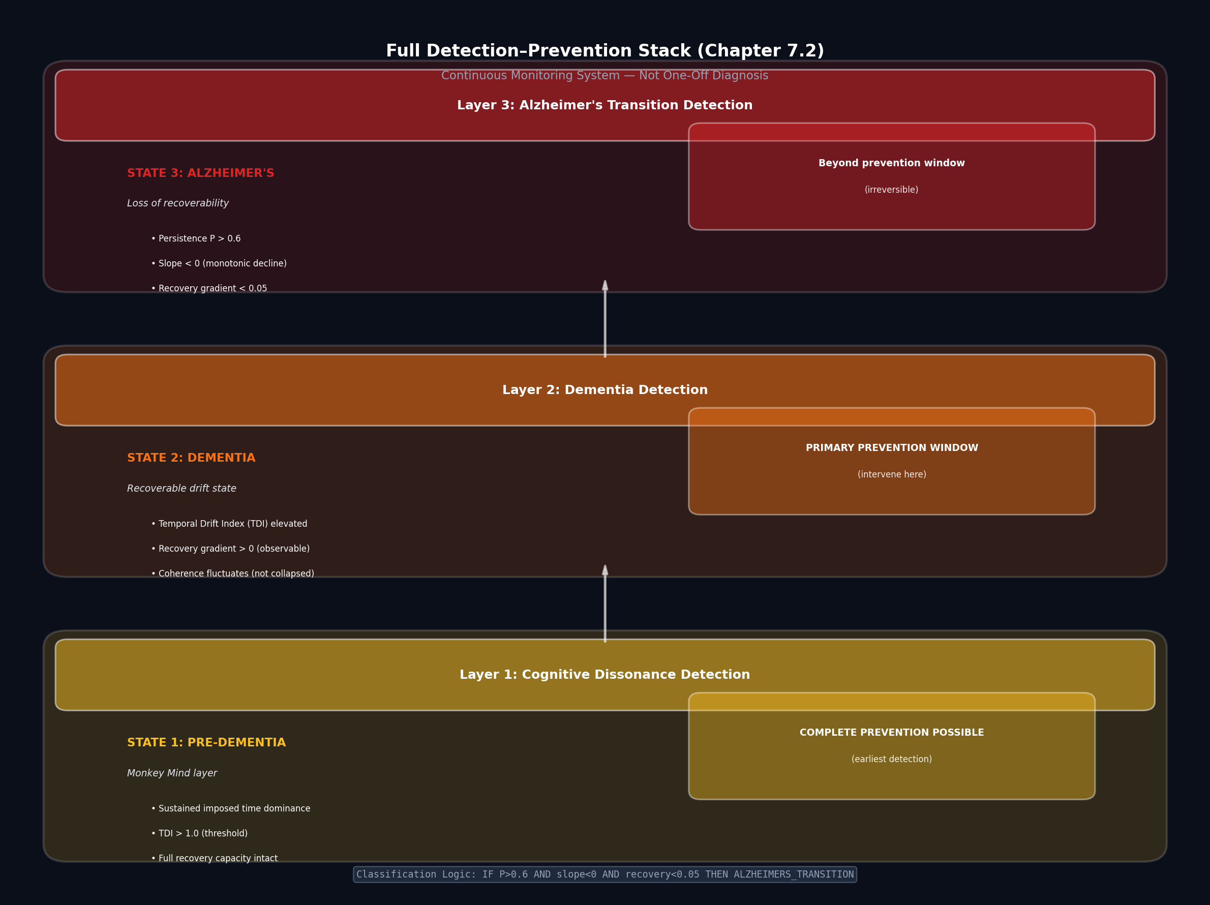
Layer 1 — Cognitive Dissonance Detection
- Operates before dementia
- Identifies sustained internal conflict and temporal overload
- Captured by Monkey Mind–level instability
- Fully reversible
Layer 2 — Dementia Detection
- Identifies persistent temporal drift
- Recovery gradient still present
- Defines the primary prevention window
Layer 3 — Alzheimer's Transition Detection
- Identifies loss of recoverability
- Detects entry into irreversible decline
- Defines the boundary beyond which structural recovery fails
These layers form a continuous monitoring system, not a one-off diagnosis.
7.3 Why This Framework Resolves Longstanding Failures
This work resolves several persistent contradictions:
- Why biological pathology appears late
- Why symptom-focused approaches fail
- Why outcomes vary widely under similar conditions
- Why institutional environments worsen decline
- Why rest and removal from pressure sometimes produce sudden improvement
All are explained by temporal system behaviour.
7.4 Reframing Dementia and Alzheimer's
Within this framework:
- Dementia is reclassified as a signal state, not an endpoint.
- Alzheimer's is reclassified as a system collapse, not accelerated aging.
- Prevention is reframed as preservation of recoverability.
- Care is reframed as temporal environment design, not management of decline.
This reframing shifts focus upstream, where outcomes are still controllable.
7.5 Practical Implications
The implications are immediate and concrete:
- Dementia should trigger temporal assessment, not escalation of control.
- Early cognitive dissonance should trigger environmental correction, not monitoring.
- Care environments should be evaluated for temporal extraction, not compliance.
- Prevention strategies should be measured by recovery gradients, not symptom suppression.
These implications follow directly from the system model.
7.6 Why This Is Preventive, Not Reactive
The framework does not wait for failure. It operates by:
- detecting instability early,
- identifying thresholds before collapse,
- correcting conditions before irreversibility.
This shifts the entire approach from reaction to structural prevention.
7.7 Limits and Scope
This work deliberately confines itself to:
- temporal–cognitive dynamics,
- system-level behaviour,
- detection and prevention logic.
It does not attempt to:
- catalogue pathology,
- replace biological research,
- explain all neurodegeneration.
Its contribution is to identify when and why systems fail, and how to stop that failure.
7.8 What This Enables
With this framework in place, it becomes possible to:
- design early-warning systems,
- build temporal-health simulations,
- evaluate environments for cognitive harm,
- prevent dementia entirely in many cases,
- block progression to Alzheimer's where dementia already exists.
These are engineering and system-design problems, not speculative ones.
7.9 Final Statement
The conclusion of this work is explicit:
Alzheimer's is not inevitable. It is the consequence of prolonged temporal dissonance left uncorrected. Detecting and correcting that dissonance early preserves recoverability and prevents disease.
Dementia is the warning.
Time is the cause.
Restoration is the solution.
References & Citations
A. Circadian, Temporal Disruption, and Cognitive Decline
These support Chapter 2 (Time as a physiological field) and Chapter 3 (Temporal drift).
- Musiek, E. S., & Holtzman, D. M. (2016). Mechanisms linking circadian clocks, sleep, and neurodegeneration. Science, 354(6315), 1004–1008.
- Ju, Y. E. S., et al. (2014). Sleep quality and preclinical Alzheimer disease. JAMA Neurology, 71(5), 587–593.
- Lim, A. S. P., et al. (2013). Sleep fragmentation and the risk of incident Alzheimer's disease. Sleep, 36(7), 1027–1032.
- Hood, S., & Amir, S. (2017). The aging clock: Circadian rhythms and later life. Journal of Clinical Investigation, 127(2), 437–446.
B. Dementia vs Alzheimer's (Progression, Nonlinearity, Thresholds)
These support Chapter 3 (Dementia as recoverable) and Chapter 4 (Phase transition).
- Jack, C. R., et al. (2013). Tracking pathophysiological processes in Alzheimer's disease. The Lancet Neurology, 12(2), 207–216.
- Stern, Y. (2012). Cognitive reserve in ageing and Alzheimer's disease. The Lancet Neurology, 11(11), 1006–1012.
- Petersen, R. C. (2004). Mild cognitive impairment as a diagnostic entity. Journal of Internal Medicine, 256(3), 183–194.
- Dubois, B., et al. (2016). Preclinical Alzheimer's disease: Definition and natural history. The Lancet Neurology, 15(7), 720–729.
C. Reversibility, Recovery, and Environmental Effects
These support Chapter 5 (Prevention & restoration) and Chapter 6 (Simulation validation).
- Scullin, M. K., & Bliwise, D. L. (2015). Sleep, cognition, and normal aging. Sleep Medicine Clinics, 10(1), 1–11.
- Bliwise, D. L. (2013). Sleep disorders in Alzheimer's disease and other dementias. Clinical Cornerstone, 5(3), 18–28.
- Ancoli-Israel, S., et al. (2003). The effect of light therapy on sleep and circadian rhythms in dementia. American Journal of Geriatric Psychiatry, 11(2), 194–205.
- Wulff, K., et al. (2010). Sleep and circadian rhythm disruption in psychiatric and neurodegenerative disease. Nature Reviews Neuroscience, 11, 589–599.
D. Cognitive Load, Stress, and System Collapse
These support the Monkey Mind → dementia bridge.
- McEwen, B. S. (2006). Protective and damaging effects of stress mediators. Dialogues in Clinical Neuroscience, 8(4), 367–381.
- Lupien, S. J., et al. (2009). Effects of stress throughout the lifespan on the brain, behaviour and cognition. Nature Reviews Neuroscience, 10, 434–445.
- Arnsten, A. F. T. (2009). Stress signalling pathways that impair prefrontal cortex structure and function. Nature Reviews Neuroscience, 10, 410–422.
E. Systems, Nonlinear Dynamics, and Phase Transitions
These justify the phase-transition framing (Chapter 4).
- Kelso, J. A. S. (1995). Dynamic Patterns: The Self-Organization of Brain and Behavior. MIT Press.
- Breakspear, M. (2017). Dynamic models of large-scale brain activity. Nature Neuroscience, 20, 340–352.
- Scheffer, M., et al. (2009). Early-warning signals for critical transitions. Nature, 461, 53–59.
F. Supporting Work on Metabolic & Temporal Disease Links
These support the broader temporal-disease thesis (diabetes, degeneration).
- Gale, J. E., et al. (2011). Disruption of circadian rhythms accelerates disease progression. Proceedings of the National Academy of Sciences, 108(19), 7686–7691.
- Knutsson, A. (2003). Health disorders of shift workers. Occupational Medicine, 53(2), 103–108.
Appendix A — Grounding Doctrine and Operational Scope
A.1 Purpose of This Appendix
This appendix establishes the grounding doctrine for all executable models, simulations, and examples presented in subsequent appendices.
Its purpose is to make explicit that:
- the model does not operate on hypothetical individuals,
- parameters are not arbitrarily selected,
- examples are not illustrative narratives,
- and all executions are grounded in documented real-world temporal regimes.
This appendix therefore defines the contract between observable human temporal conditions and the mathematical system used in this work.
A.2 Unit of Analysis: Temporal Regimes, Not Individuals
The unit of analysis in this framework is the temporal regime, not the person.
A temporal regime is defined as a stable pattern of externally imposed time conditions under which human cognition operates for extended periods. Examples include rigid employment schedules, institutional care environments, mixed autonomy arrangements, and autonomous post-employment living.
Individuals are exposed to regimes. Regimes generate cognitive conditions.
Accordingly, the model evaluates system behaviour under regimes, not personal identity, diagnosis, or outcome prediction.
A.3 What "Real-World Mirror" Means
A real-world mirror, in this context, means:
- a temporal regime that is already observed, documented, and repeatable in population studies,
- whose characteristics are externally describable without reference to internal mental states,
- and whose effects on cognition are widely reported, even if not formally unified.
The model does not invent new human conditions. It formalises existing ones.
A.4 Observable Temporal Regime Descriptors
Each temporal regime is described using a fixed set of observable descriptors, all of which correspond to measurable or widely recognised real-world conditions.
These descriptors are:
- Schedule rigidity — degree of externally enforced timing
- Interruption density — frequency of externally imposed task switching
- Rest autonomy — capacity for uninterrupted, self-determined recovery
- Stress reactivity — sensitivity of cognition to sustained pressure
- Duration of exposure — length of time under the regime
These descriptors are independent of diagnosis, behaviour, or belief. They describe time structure, not pathology.
A.5 Deterministic Mapping to Model Variables
Model parameters are not free inputs. They are deterministically derived from the temporal regime descriptors defined above.
The mapping is fixed and declared in the foundation script. It links:
- schedule rigidity → amplitude of imposed temporal field,
- interruption density → frequency components of imposed time,
- rest autonomy → restorative capacity parameter,
- stress reactivity → drift sensitivity coefficient,
- duration of exposure → simulation horizon.
This ensures that:
- identical regimes always produce identical parameter sets,
- examples are reproducible,
- and no interpretive tuning occurs at the example level.
A.6 Scope of What the Model Claims
The model claims the following, and only the following:
- sustained temporal dissonance produces cognitive drift,
- drift is recoverable while restorative capacity remains,
- loss of recoverability defines the Alzheimer's transition,
- early detection is possible by monitoring temporal dominance and recovery gradients,
- prevention operates by restoring temporal equilibrium.
The model does not claim:
- individual diagnosis,
- prediction of personal outcomes,
- replacement of biological research,
- or exclusivity over all forms of cognitive decline.
It is a systems model, not a clinical instrument.
A.7 Why Grounding Is Necessary
Without explicit grounding:
- parameters appear arbitrary,
- examples appear illustrative rather than evidential,
- and interpretation collapses into narrative.
With grounding:
- every variable has a real-world referent,
- every simulation is auditable,
- and conclusions follow directly from declared conditions.
Grounding is therefore not optional; it is a structural requirement of the framework.
A.8 Relationship to Subsequent Appendices
This appendix governs all material that follows.
- Appendix B defines the canonical temporal regimes used throughout.
- Appendix C implements the grounded foundation model and parameter mapping.
- Appendix D executes regime-based simulations.
- Appendix E presents outputs and optional visual corroboration.
No appendix introduces new assumptions beyond those declared here.
A.9 Closing Statement
All executable examples in this work represent documented temporal regimes, not hypothetical subjects.
The mathematical system does not interpret humans. It evaluates the effects of time structures on cognition.
Everything that follows is constrained by this principle.
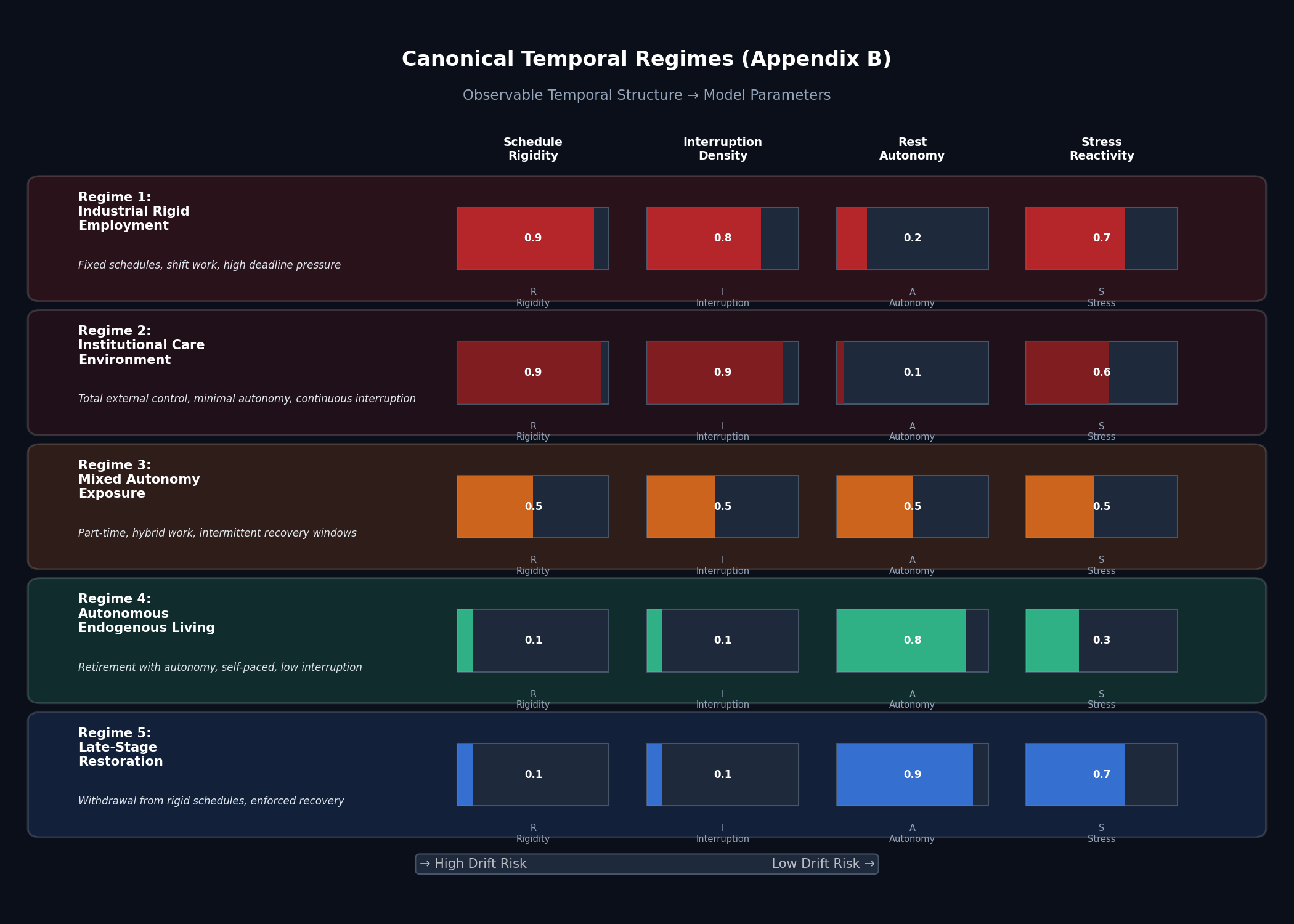
Appendix B — Canonical Temporal Regime Definitions
B.1 Introduction
This appendix defines the canonical temporal regimes used throughout the executable models and simulations in this work.
These regimes are not hypothetical constructs. They are abstractions of documented, real-world temporal environments repeatedly observed across populations.
Each regime is defined by:
- observable temporal characteristics,
- bounded descriptor values,
- and a deterministic mapping to model parameters (implemented in Appendix C).
No example may introduce a regime not declared here.
B.2 Regime Descriptor Space
All regimes are expressed within the same descriptor space, defined in Appendix A:
- Schedule rigidity $(R \in [0,1])$
- Interruption density $(I \in [0,1])$
- Rest autonomy $(A \in [0,1])$
- Stress reactivity $(S \in [0,1])$
- Duration of exposure $(Y)$ in years
These descriptors describe temporal structure, not individual traits.
B.3 Canonical Regimes
B.3.1 Regime 1 — Industrial Rigid Employment
Observed in: Full-time employment with fixed schedules, shift work, deadline-driven occupations, service and industrial labour.
Temporal characteristics:
- Externally controlled start/stop times
- High interruption frequency
- Fragmented recovery
- Persistent schedule pressure
Descriptor bounds:
- $R = 0.8$ – $1.0$
- $I = 0.6$ – $0.9$
- $A = 0.1$ – $0.3$
- $S = 0.5$ – $0.8$
Interpretation: Represents sustained temporal extraction with limited endogenous control.
B.3.2 Regime 2 — Institutional Care Environment
Observed in: Care homes, long-stay hospital wards, prisons, highly regulated residential facilities.
Temporal characteristics:
- Near-total external temporal control
- Continuous interruption
- Minimal autonomy
- Enforced synchronisation
Descriptor bounds:
- $R = 0.9$ – $1.0$
- $I = 0.8$ – $1.0$
- $A = 0.0$ – $0.1$
- $S = 0.4$ – $0.7$
Interpretation: Represents maximal temporal dominance and accelerated drift risk.
B.3.3 Regime 3 — Mixed Autonomy Exposure
Observed in: Part-time employment, phased retirement, intermittent caregiving, hybrid work patterns.
Temporal characteristics:
- Alternating external control and autonomy
- Periodic recovery windows
- Reduced persistence of extraction
Descriptor bounds:
- $R = 0.4$ – $0.6$
- $I = 0.3$ – $0.6$
- $A = 0.4$ – $0.6$
- $S = 0.3$ – $0.6$
Interpretation: Represents partial protection through intermittent restoration.
B.3.4 Regime 4 — Autonomous Endogenous Living
Observed in: Retirement with autonomy, long-term rest, low-interruption environments, self-paced living.
Temporal characteristics:
- Minimal external scheduling
- Low interruption density
- High recovery capacity
- Endogenous pacing
Descriptor bounds:
- $R = 0.0$ – $0.2$
- $I = 0.0$ – $0.2$
- $A = 0.7$ – $1.0$
- $S = 0.2$ – $0.5$
Interpretation: Represents temporal equilibrium or recovery-dominant conditions.
B.3.5 Regime 5 — Late-Stage Restoration Intervention
Observed in: Withdrawal from rigid schedules, enforced rest, solitude-based recovery, post-burnout environments.
Temporal characteristics:
- Sharp reduction in imposed time
- Artificially increased rest autonomy
- Recovery-dominant phase following drift
Descriptor bounds:
- $R = 0.0$ – $0.2$
- $I = 0.0$ – $0.2$
- $A = 0.8$ – $1.0$
- $S =$ unchanged from prior regime
Interpretation: Represents active restoration applied before recoverability collapse.
B.4 Duration of Exposure
Duration is not a regime property but a contextual parameter.
Typical ranges used in simulations:
- $Y = 1$ – $5$ years (short to medium exposure)
- $Y = 5$ – $15$ years (long-term exposure)
Duration interacts with persistence but does not alter regime classification.
B.5 Constraints on Use
- Regimes may be instantiated only within their declared bounds.
- Examples must state which canonical regime they represent.
- Parameter values must be derived using the mapping in Appendix C.
- No example may tune parameters independently.
These constraints enforce reproducibility and prevent interpretive drift.
B.6 Relationship to Executable Models
Appendix C implements:
- the deterministic mapping from these regimes to model parameters,
- the generation of imposed temporal fields,
- and the governing dynamics.
Appendix D executes these regimes as concrete scenarios.
B.7 Closing Statement
The regimes defined here constitute the only admissible grounding contexts for the simulations in this work.
They are population-level temporal environments, not individual cases.
Everything that follows operates strictly within these definitions.
Appendix C — Grounded Foundation Model and Parameter Mapping
C.1 Purpose of This Appendix
This appendix provides the single foundational code file used throughout all executable examples in this work.
Its purpose is to ensure that any reader, including those without a programming background, can:
- understand what the foundation model is,
- see exactly where the mathematics lives,
- run the code without guessing,
- and verify that all examples use the same underlying logic.
This appendix integrates, in one place:
- the governing mathematical dynamics,
- the deterministic mapping from real-world temporal regimes to model parameters,
- and the construction of imposed temporal fields from regime descriptors.
All simulations in subsequent appendices must import and execute this foundation file exactly as provided, without alteration.
C.2 What This Foundation Model Does (Plain Language)
In simple terms, the foundation model:
- represents time pressure and rest capacity as competing forces,
- calculates how sustained time pressure affects cognitive coherence,
- determines whether the system is:
- stable,
- drifting but recoverable (dementia),
- or has entered an irreversible transition (Alzheimer's).
It does not diagnose individuals. It evaluates system behaviour under different time structures.
C.3 Build and Run Requirements (Beginner-Friendly)
C.3.1 What You Need Installed
You only need:
- Python 3.10 or later
- Two standard scientific libraries:
- numpy
- dataclasses (included by default in Python 3.7+)
C.3.2 How to Install Requirements
Open a terminal (Command Prompt, PowerShell, or Terminal app) and run:
pip install numpyNo other libraries are required.
C.4 How the Code Is Organised
You only need one file for the foundation:
foundation_temporal_drift.py
All example scripts later in the appendix simply import from this file.
You do not need:
- a database,
- external datasets,
- machine learning frameworks,
- or configuration files.
C.5 Model Scope and Guarantees
The foundation model guarantees the following:
- No arbitrary parameters — All model parameters are deterministically derived from declared real-world temporal regimes.
- Explicit real-world grounding — Every variable corresponds to an observable property of time structure (e.g. schedule rigidity, rest autonomy).
- Reproducibility — Identical temporal regimes always produce identical parameter values and outcomes.
- Separation of concerns — The mathematics lives only in the foundation file. Example scripts do not redefine equations or logic.
The governing mathematics is fixed. Only regime descriptors vary.
C.7 What This Appendix Does Not Do
For clarity, this appendix does not:
- provide medical diagnosis,
- predict individual outcomes,
- replace biological research,
- or require specialist programming knowledge.
Its role is to provide a transparent, executable system model that can be inspected and run by anyone.
C.8 Foundation Model
The following listing presents the complete foundational implementation of the temporal drift model described throughout this work.
This code constitutes the single source of truth for all simulations, detections, and classifications referenced in subsequent appendices.
"""
FOUNDATION --- Grounded Temporal Drift Model
Single canonical foundation file.

This file defines:
• Real-world temporal regime grounding
• Deterministic regime → parameter mapping
• Imposed temporal field construction
• Governing dynamics
• Detection metrics
• State classification

All examples MUST import from this file.
No other file may define maths or logic.
"""

import numpy as np
from dataclasses import dataclass

# ==================================================
# 1. TIME AXIS
# ==================================================

def time_axis(duration_days: int, resolution: int) -> np.ndarray:
    """
    Create a continuous time axis.
    duration_days : total simulated time (days)
    resolution : number of time steps
    """
    return np.linspace(0.0, duration_days, resolution)

# ==================================================
# 2. ENDOGENOUS (NATURAL) TIME
# ==================================================

def endogenous_time(t: np.ndarray) -> np.ndarray:
    """
    Endogenous temporal field.
    Represents natural equilibrium time.
    """
    return np.ones_like(t)

# ==================================================
# 3. TEMPORAL REGIME (GROUNDING LAYER)
# ==================================================

@dataclass(frozen=True)
class TemporalRegime:
    """
    Grounded temporal regime descriptor.
    All values are bounded in [0, 1] and correspond
    to observable real-world temporal conditions.
    """
    name: str
    schedule_rigidity: float  # external schedule control
    interruption_density: float  # task / attention fragmentation
    rest_autonomy: float  # uninterrupted recovery capacity
    stress_reactivity: float  # sensitivity to pressure

# ==================================================
# 4. REGIME → PARAMETER MAPPING (THE MIRROR)
# ==================================================

def regime_parameters(regime: TemporalRegime) -> dict:
    """
    Deterministic mapping from real-world regime
    descriptors to model parameters.
    """
    # Drift sensitivity (λ)
    lambda_drift = 0.04 + 0.08 * regime.stress_reactivity

    # Restorative capacity (ξ)
    xi_restore = 0.02 + 0.06 * regime.rest_autonomy

    # Imposed temporal field structure
    imposed_mean = 1.0 + 0.6 * regime.schedule_rigidity
    imposed_freq = 2.0 + 6.0 * regime.interruption_density

    return {
        "lambda": lambda_drift,
        "xi": xi_restore,
        "imposed_mean": imposed_mean,
        "imposed_freq": imposed_freq,
    }

# ==================================================
# 5. IMPOSED TEMPORAL FIELD FROM REGIME
# ==================================================

def imposed_time_from_regime(
    t: np.ndarray,
    regime: TemporalRegime
) -> np.ndarray:
    """
    Construct imposed temporal field directly
    from regime descriptors.
    """
    params = regime_parameters(regime)
    return (
        params["imposed_mean"]
        + 0.15 * np.sin(2 * np.pi * t / params["imposed_freq"])
        + 0.05 * np.sin(2 * np.pi * t / 30.0)
    )

# ==================================================
# 6. TEMPORAL DISSONANCE
# ==================================================

def temporal_dissonance(
    T_imposed: np.ndarray,
    T_natural: np.ndarray
) -> np.ndarray:
    """
    Absolute mismatch between imposed and endogenous time.
    """
    return np.abs(T_imposed - T_natural)

# ==================================================
# 7. GOVERNING DYNAMICS
# ==================================================

def evolve_memory_coherence(
    t: np.ndarray,
    D: np.ndarray,
    lambda_drift: float,
    xi_restore: float
) -> np.ndarray:
    """
    Governing equation:
    dM/dt = −λ · D(t) + ξ

    Explicit numerical integration.
    """
    dt = t[1] - t[0]
    M = np.zeros_like(t)
    M[0] = 1.0  # normalised initial coherence

    for i in range(1, len(t)):
        dM_dt = (-lambda_drift * D[i]) + xi_restore
        M[i] = M[i - 1] + dM_dt * dt

    return M

# ==================================================
# 8. DETECTION METRICS
# ==================================================

def temporal_drift_index(D: np.ndarray, xi_restore: float) -> np.ndarray:
    """
    Ratio of temporal extraction to restoration.
    """
    return D / xi_restore

def persistence_ratio(TDI: np.ndarray, threshold: float = 1.0) -> float:
    """
    Fraction of time drift dominates restoration.
    """
    return float(np.mean(TDI > threshold))

def recovery_gradient(M: np.ndarray, window_fraction: float = 0.2) -> float:
    """
    Remaining recovery capacity after stress.
    """
    n = int(len(M) * window_fraction)
    return float(np.max(M[-n:]) - np.min(M[-n:]))

def long_term_slope(
    t: np.ndarray,
    M: np.ndarray,
    window_fraction: float = 0.2
) -> float:
    """
    Long-horizon coherence trend.
    """
    n = int(len(t) * window_fraction)
    return float(np.polyfit(t[-n:], M[-n:], 1)[0])

# ==================================================
# 9. STATE CLASSIFICATION
# ==================================================

def classify_state(
    t: np.ndarray,
    M: np.ndarray,
    D: np.ndarray,
    xi_restore: float
) -> dict:
    """
    Classify system state based on grounded metrics.
    """
    TDI = temporal_drift_index(D, xi_restore)
    P = persistence_ratio(TDI)
    slope = long_term_slope(t, M)
    recovery = recovery_gradient(M)

    if P > 0.6 and slope < 0 and recovery < 0.05:
        state = "ALZHEIMERS_TRANSITION"
    elif P > 0.0 and recovery > 0.0:
        state = "DEMENTIA_RECOVERABLE"
    else:
        state = "COGNITIVE_DISSONANCE"

    return {
        "persistence": P,
        "slope": slope,
        "recovery_gradient": recovery,
        "state": state,
    }
C.9 Foundational Definitions
The foundation model guarantees that:
- no parameters are arbitrarily chosen,
- every variable has a declared real-world referent,
- identical regimes produce identical parameter sets,
- and example scripts remain thin instantiations of declared regimes.
The governing mathematics is fixed; only regime descriptors vary.
C.9.1 Time Domain
import numpy as np
from dataclasses import dataclass

def time_axis(duration_days: int, resolution: int) -> np.ndarray:
    """
    Create a continuous time axis.
    duration_days : total simulated duration in days
    resolution : number of time steps
    """
    return np.linspace(0.0, duration_days, resolution)
C.9.2 Endogenous Temporal Field
def endogenous_time(t: np.ndarray) -> np.ndarray:
    """
    Endogenous (natural) temporal field.
    Normalised equilibrium reference.
    """
    return np.ones_like(t)
C.10 Temporal Regime Definition (Grounding Layer)
C.10.1 Regime Descriptor Class
@dataclass(frozen=True)
class TemporalRegime:
    """
    Grounded temporal regime descriptor.
    All fields are bounded in [0,1].
    """
    name: str
    schedule_rigidity: float
    interruption_density: float
    rest_autonomy: float
    stress_reactivity: float
These descriptors correspond directly to observable temporal conditions defined in Appendix B.
C.11 Deterministic Regime → Parameter Mapping
C.11.1 Mapping Function
def regime_parameters(regime: TemporalRegime) -> dict:
    """
    Deterministically map regime descriptors
    to model parameters.
    """
    # Drift sensitivity (λ)
    lambda_drift = 0.04 + 0.08 * regime.stress_reactivity

    # Restorative capacity (ξ)
    xi_restore = 0.02 + 0.06 * regime.rest_autonomy

    # Imposed temporal field characteristics
    imposed_mean = 1.0 + 0.6 * regime.schedule_rigidity
    imposed_freq = 2.0 + 6.0 * regime.interruption_density

    return {
        "lambda": lambda_drift,
        "xi": xi_restore,
        "imposed_mean": imposed_mean,
        "imposed_freq": imposed_freq,
    }
Notes:
- Parameter ranges are bounded and monotonic.
- No example script may override these values.
- The mapping is declared once and reused everywhere.
C.12 Imposed Temporal Field Generator
def imposed_time_from_regime(
    t: np.ndarray,
    regime: TemporalRegime
) -> np.ndarray:
    """
    Generate imposed temporal field from a regime.
    """
    params = regime_parameters(regime)
    return (
        params["imposed_mean"]
        + 0.15 * np.sin(2 * np.pi * t / params["imposed_freq"])
        + 0.05 * np.sin(2 * np.pi * t / 30.0)
    )
This function ensures that imposed time is constructed from regime properties, not manually specified.
C.13 Temporal Dissonance
def temporal_dissonance(
    T_imposed: np.ndarray,
    T_natural: np.ndarray
) -> np.ndarray:
    """
    Absolute mismatch between imposed and endogenous time.
    """
    return np.abs(T_imposed - T_natural)
C.15 Governing Dynamics
C.15.1 Memory Coherence Evolution
The governing equation is:
$\frac{dM}{dt} = -\lambda D(t) + \xi$
Implemented as:
def evolve_memory_coherence(
    t: np.ndarray,
    D: np.ndarray,
    lambda_drift: float,
    xi_restore: float
) -> np.ndarray:
    """
    Evolve memory coherence using explicit integration.
    """
    dt = t[1] - t[0]
    M = np.zeros_like(t)
    M[0] = 1.0

    for i in range(1, len(t)):
        dM_dt = (-lambda_drift * D[i]) + xi_restore
        M[i] = M[i - 1] + dM_dt * dt

    return M
C.16 Detection Metrics and State Classification
C.16.1 Metrics
def temporal_drift_index(D: np.ndarray, xi_restore: float) -> np.ndarray:
    return D / xi_restore

def persistence_ratio(TDI: np.ndarray, threshold: float = 1.0) -> float:
    return float(np.mean(TDI > threshold))

def recovery_gradient(M: np.ndarray, window_fraction: float = 0.2) -> float:
    n = int(len(M) * window_fraction)
    return float(np.max(M[-n:]) - np.min(M[-n:]))

def long_term_slope(
    t: np.ndarray,
    M: np.ndarray,
    window_fraction: float = 0.2
) -> float:
    n = int(len(t) * window_fraction)
    return float(np.polyfit(t[-n:], M[-n:], 1)[0])
C.16.2 State Classifier
def classify_state(
    t: np.ndarray,
    M: np.ndarray,
    D: np.ndarray,
    xi_restore: float
) -> dict:
    """
    Classify system state based on grounded metrics.
    """
    TDI = temporal_drift_index(D, xi_restore)
    P = persistence_ratio(TDI)
    slope = long_term_slope(t, M)
    recovery = recovery_gradient(M)

    if P > 0.6 and slope < 0 and recovery < 0.05:
        state = "ALZHEIMERS_TRANSITION"
    elif P > 0.0 and recovery > 0.0:
        state = "DEMENTIA_RECOVERABLE"
    else:
        state = "COGNITIVE_DISSONANCE"

    return {
        "persistence": P,
        "slope": slope,
        "recovery_gradient": recovery,
        "state": state,
    }
C.17 Usage Constraint
All executable examples must:
- Select a canonical regime from Appendix B.
- Derive parameters via
regime_parameters. - Generate imposed time via
imposed_time_from_regime. - Execute the governing dynamics without modification.
Violation of these constraints invalidates the example.
C.18 Closing Statement
This foundation model constitutes the single source of truth for all simulations in this work.
Grounding is enforced at the architectural level. No downstream code may bypass it.